NanoFlow: Training Flow-Matching Models from Scratch on a Budget

NanoFlow

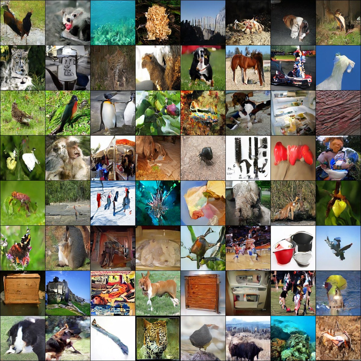
Before diving into the post, take a look at a training sample logged early in training, to illustrate some of the funny (and sometimes horrifying) model outputs:

At least you can kind of tell it's a dog, right?

Don’t worry, it’ll get better (slightly).

Introduction

I’m sharing what I learned training conditional flow-matching image models from scratch. All the core training and sampling here use ODE flow matching, although later we use the SDE interpretation of Flow matching during Flow-GRPO post-training. I was partially inspired by nanochat, specifically the naming and the initial $100 budget.

The purpose of this project was to experiment with training conditional flow-matching models from scratch on a “hobbyist budget”. My requirements were:

• Cheap enough to experiment locally, or on a small budget. I initially planned for about $100 in GPU compute, but the final ImageNet-256 model cost $210.45 at $3.30/H100-hour. The models leading up to that were much cheaper. Most earlier stages were trained locally on a consumer GPU (16GB VRAM) or my MacBook Pro GPU (M4 Pro).
• Demonstrate how to do post-training with a simple reward function (via Flow-GRPO).
• Minimal dependencies. Writing from scratch, and being able to read all of the code in a single codebase, are better for learning. I did end up importing diffusers, but only to use a pre-trained VAE for Latent Diffusion Model (LDM) training. Other dependencies are mainly for training infrastructure.
• Provide a visual demonstration of how scaling up flow-matching models can allow for modeling more complex distributions, mostly through higher resolution and more semantic classes.

Here are the flow-matching models we trained, from simplest to most complex:

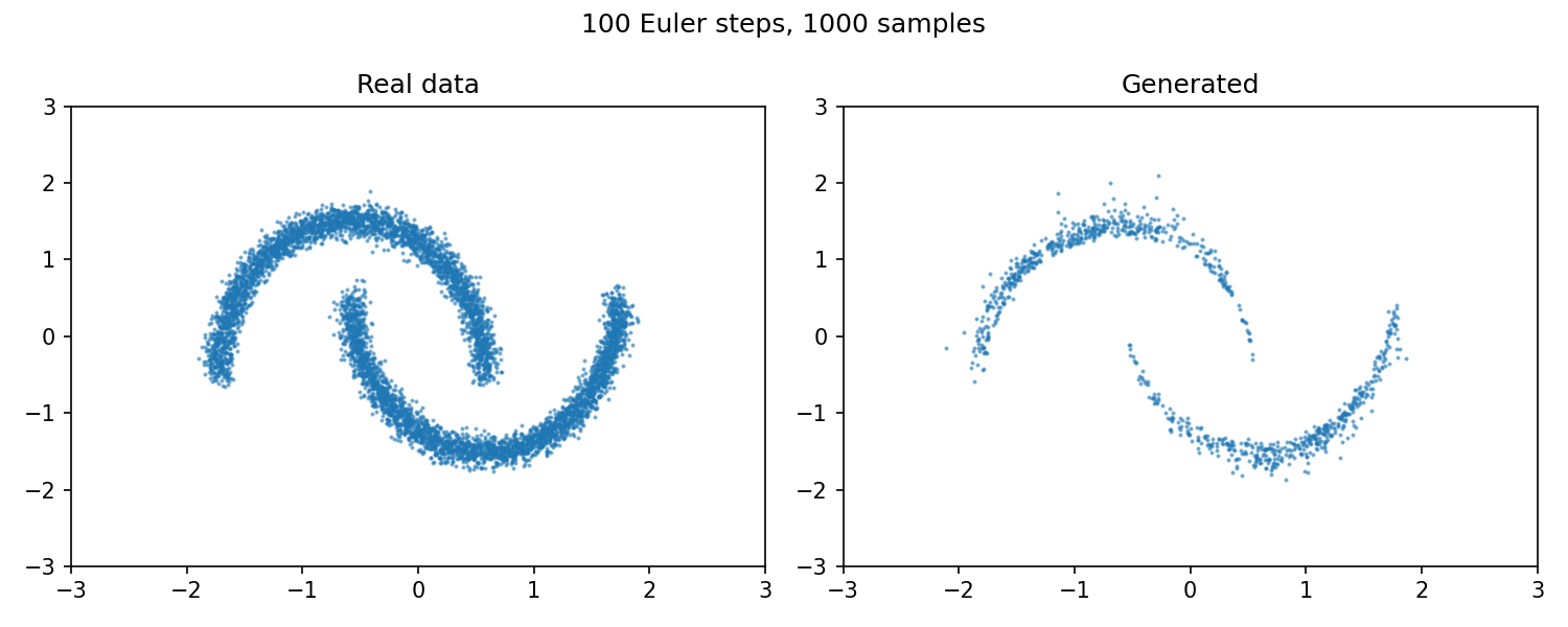
1. Generated Moons synthetic data (low-dimensional).
2. Fashion-MNIST: 70,000 total samples, 10 classes, 60,000 train / 10,000 test, 28x28 grayscale. This stage also includes two toy RL objectives: “pantsiness” and “compressibility”.
3. CIFAR-10: 60,000 total samples, 10 classes, 50,000 train / 10,000 test, 32x32 RGB. This has much broader semantic variety than Fashion-MNIST.
4. ImageNet-256: 1000 classes, ~1.4M samples, 256x256 RGB. Initially we trained a latent U-Net model, but the quality was poor, so we scaled up to a DiT-style latent model.

Code

All code for training, sampling, and job submission is in my NanoFlow repository. Some throwaway YAML files for launching SkyPilot jobs on cloud GPUs are not checked in, but the documentation should be self-explanatory on how to launch training runs locally or via SkyPilot jobs.

At a high level, the codebase is organized around a few small, mostly independent pieces:

• Configs: configs/ contains Hydra configs for datasets, models, training hyperparameters, rewards, metrics, solvers, and experiment presets. Most runs are launched by selecting an experiment=... preset and overriding a few fields from the CLI.
• Data: datasets.py contains the dataset wrappers for Moons, Fashion-MNIST, CIFAR-10, ImageNet-256 images, and ImageNet-256 VAE latents. The ImageNet latent-cache scripts live under scripts/.
• Models: models.py contains the MLP and U-Net models used for Moons, Fashion-MNIST, and CIFAR-10. models_dit.py contains the DiT-style ImageNet latent models, including the patch mixer, deferred token masking, and MoE layers.
• Training and sampling: flow.py defines the probability path, train.py implements the flow-matching training loop, inference.py implements sampling, and ode_solvers.py contains Euler/Heun solvers.
• Post-training: train_grpo.py and rl/ contain the Flow-GRPO implementation, including SDE rollouts, group-relative advantages, KL penalties, and reward functions.
• Cloud training infrastructure (SkyPilot, RunPod): cloud/runpod/, scripts/sky_runpod_chain.py, and the docs/imagenet*.md files contain the RunPod/SkyPilot job chains, cache-preparation commands, and ImageNet eval workflows.
• Experiments: experiments/ contains write-ups describing how to reproduce each experiment mentioned below.

Flow Matching Background

All of our models are trained with the conditional flow-matching loss. We use $x_1 \sim p_\text{data}$ time convention. The models are trained to predict the flow vector field

\[\mathcal{L}(\theta) = \mathbb{E}_{(x_1, c) \sim p_\text{data}, \epsilon \sim \mathcal{N}(0, \mathbf{I}), t \sim \mathcal{U}(0,1)} \lbrack \|u_\theta(x_t, t, c) - u_t^\text{target} \|^2\rbrack\]

We use the Conditional Optimal Transport (CondOT) probability path, defined as follows:

\[x_t = (1-t)\epsilon + t x_1\] \[u_t^\text{target} = x_1 - \epsilon\]

See our previous post on probability paths for visualizations of the CondOT path.

The relevant modules for training the conditional flow vector fields and sampling from them are listed below:

• flow.py — CondOT interpolation and target velocity.
• train.py — model training, MSE / masked-MSE loss, checkpoint/resume, post-train sampling.
• inference.py — ODE sampling and classifier-free guidance sampling.
• ode_solvers.py — Euler and Heun latent ODE solvers.

We also trained the class-conditional models with classifier-free guidance (CFG). During training, we randomly replace the class label with a learned null/unconditional label for a fraction of batches. At sampling time, we evaluate the model twice: once with the desired class label and once with the null label. The guided velocity is then

\[u_\text{cfg}(x_t, t, c) = u_\text{uncond}(x_t, t) + s\left(u_\text{cond}(x_t, t, c) - u_\text{uncond}(x_t, t)\right)\]

where $s$ is the guidance scale. Intuitively, this pushes samples more strongly in the direction that distinguishes the requested class from the unconditional model. In the code, null replacement rate is controlled by training.p_uncond during training and guidance_scale sets $s$ during sampling.

Summary of models & training cost

Stage	Main model	Params / active params	Approx training compute	Runtime / GPU time	Cloud GPU cost
Moons	ClassCondMLP	~70.8K	~539 GFLOPs	~37s on MPS	local / $0
Fashion-MNIST	ClassCondUNet	~0.347M	~78.6 TFLOPs for 3-epoch CFG seed; ~0.524 PFLOPs for 20-epoch baseline	~1.3 min seed; ~8.1 min baseline on MPS	local / $0
Fashion GRPO JPEG	Fashion ClassCondUNet policy	~0.347M	~0.700 PFLOPs	~11.1 min on MPS	local / $0
Fashion GRPO pantsiness	Fashion ClassCondUNet policy	~0.347M	~0.915 PFLOPs	~16.7 min on MPS	local / $0
CIFAR-10	ClassCondUNet	22.311M	~320 PFLOPs	~4.1–4.3h on RTX 4080	local / $0
ImageNet latent U-Net	latent ClassCondUNet	~89.8M	~8.4 EFLOPs	~16.5 H100-hours	~$54.45 at $3.30/H100-hour
ImageNet latent DiT/MoE	H1024 D20 E16 deferred-masking DiT/MoE	695.1M total / 314.0M active	~41 EFLOPs	63.77 H100-hours	$210.45 at $3.30/H100-hour

Stage 1: Moons

We generate 8k two-moons samples, with each crescent used as the class label for conditioning. The output is a small, very low-dimensional (2D) dataset.

Purpose: cheap 2D debugging stage for the probability path, training loop, sampling, and CFG/class conditioning.

Data & Model

• Baseline model: MLP
• CFG model: ClassCondMLP.
• Model size: ~70.8k parameters.

Code pointers:

• configs/experiment/moons.yaml
• configs/experiment/moons_cfg.yaml
• configs/dataset/moons.yaml
• configs/model/mlp.yaml
• datasets.py
• models.py

Training Recipe

• Representative 200-epoch runs: 10,000 steps, 1.28M training samples.
• Estimated compute: ~539 GFLOPs.
• Wall time: ~37 seconds on MPS.

Reproduction details live in experiments/moons.md in the NanoFlow repository.

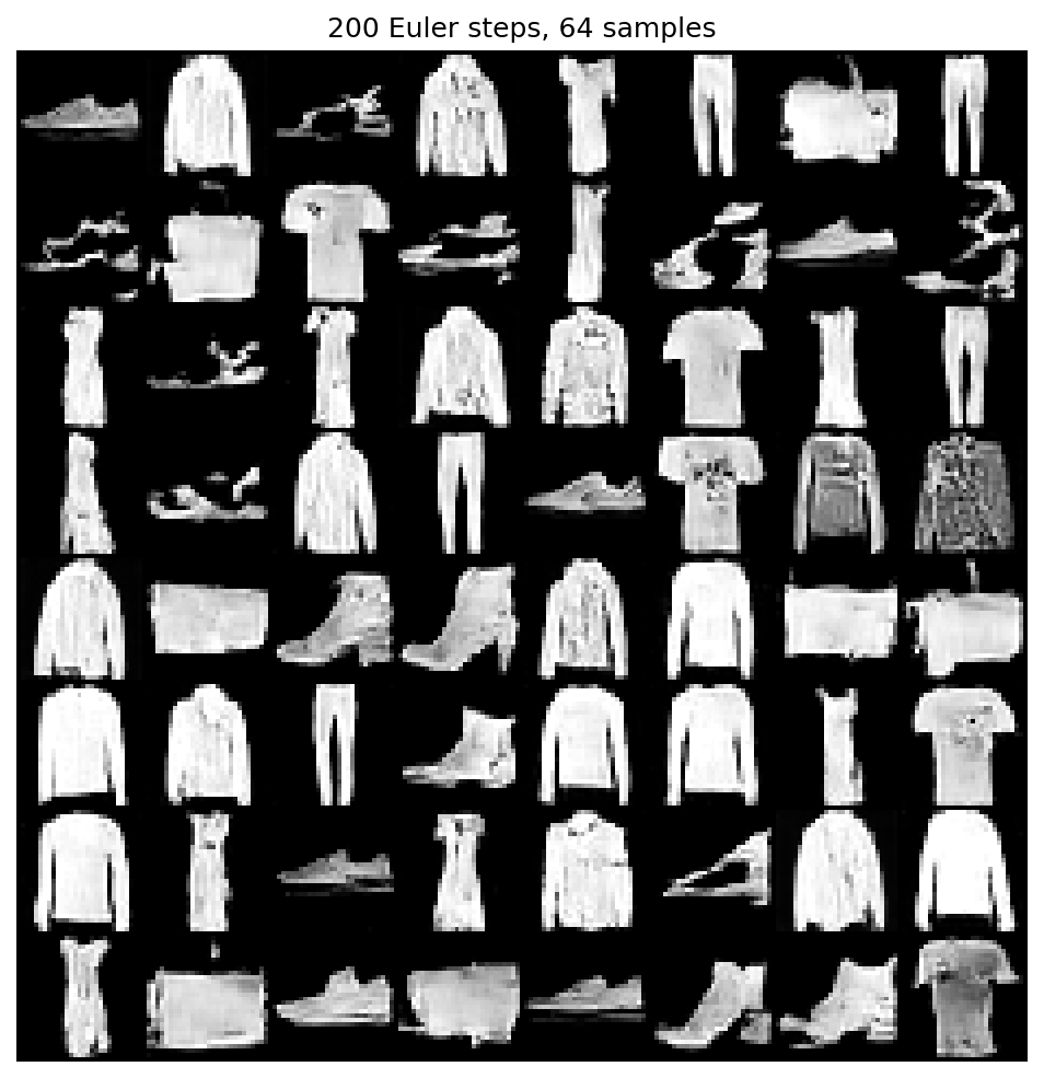
Stage 2: Fashion-MNIST

At this stage, we move on to class-conditioned image generation. Whereas the previous model was an MLP, here we moved to a U-Net architecture. We stay in pixel domain, since the training images are low resolution 28x28 grayscale. Training is runnable (both pre-training and post-training) on local MPS backend in a short time. In addition, we added some GRPO post-training stages for 2 different reward functions.

Data & Model

• Dataset: Fashion-MNIST, 70,000 total samples, 10 classes, 60,000 train / 10,000 test.
• Shape: 28x28 grayscale.
• Baseline model: small U-Net, depth 2, no attention.
• CFG model: ClassCondUNet with p_uncond=0.1.
• Model size: 347,361 parameters for the class-conditional model.

(Pre-)Training Recipe

• 20-epoch supervised baseline: 9,360 steps, 1.198M training samples.
• Estimated baseline compute: ~0.524 PFLOPs.
• Wall time: ~8.1 minutes on MPS.
• 3-epoch CFG seed for GRPO: ~78.6 TFLOPs.

Code pointers:

• configs/experiment/fashion.yaml
• configs/experiment/fashion_cfg.yaml
• configs/dataset/fashion.yaml
• configs/model/unet_fashion.yaml
• configs/model/classcond_unet_fashion.yaml
• datasets.py
• models.py

Reproduction details live in experiments/fashion_mnist.md in the NanoFlow repository.

Flow-GRPO Post-training

Post-training for image-generation models is typically used for one of several things:

• Aligning the model with human aesthetic preferences, usually via models like LAION aesthetics predictor.
• Improving prompt-image alignment.
• Character consistency.
• Style transfer.

For a small-compute setting, and without curating additional datasets, I decided it would be interesting to implement Flow-GRPO and devise some toy reward functions:

• Make everything look “pantsier” (fool a lightweight classifier into thinking every generated sample is from the Fashion-MNIST “Trouser” class).
• JPEG compression reward. The generated samples score higher if the image uses fewer bits once JPEG compression is applied.

Flow-GRPO Overview

Flow-GRPO is a policy-gradient update for flow models. It treats a denoising trajectory as an MDP where the state is the current sample, time, and condition, $s_k = (x_{t_k}, t_k, c)$, and the action is the next sample, $a_k = x_{t_{k+1}}$. In our CondOT convention, the rollout starts near noise and ends near data at $t=1$.

The Flow-GRPO paper converts the deterministic flow ODE into an SDE so each transition has a Gaussian policy density:

\[\pi_\theta(a_k \mid s_k) = \mathcal{N}(\mu_\theta^k, \sigma_k^2 \mathbf{I})\]

This makes PPO-style likelihood ratios and reference-policy KL terms well-defined. A deterministic ODE sampler would instead give degenerate transitions, making those quantities singular or uninformative. The reward is evaluated only at the terminal sample:

\[R_i = r(x_{1,i}, c_i)\]

For each prompt/class $j$, we sample a group of $G$ images and convert terminal rewards into group-relative advantages:

\[A_{j,g} = \frac{R_{j,g} - \operatorname{mean}_{g'} R_{j,g'}}{\operatorname{std}_{g'} R_{j,g'} + \epsilon}\]

The same terminal advantage is applied to every transition in that sample’s rollout. The policy-gradient loss uses a PPO-style clipped importance ratio:

\[\rho_{k,i}(\theta) = \exp\left(\log \pi_\theta(a_{k,i} \mid s_{k,i}) - \log \pi_\text{old}(a_{k,i} \mid s_{k,i})\right)\] \[\mathcal{L}_\text{PG}(\theta) = -\mathbb{E}_{k,i}\left[\min\left(\rho_{k,i} A_i, \operatorname{clip}(\rho_{k,i}, 1 - \epsilon_\text{clip}, 1 + \epsilon_\text{clip}) A_i\right)\right]\]

We regularize against a frozen reference policy with a closed-form Gaussian KL over the SDE transition means:

\[D_\text{KL}\left(\mathcal{N}(\mu_\theta^k, \sigma_k^2 \mathbf{I}) \| \mathcal{N}(\mu_\text{ref}^k, \sigma_k^2 \mathbf{I})\right) = \frac{\|\mu_\theta^k - \mu_\text{ref}^k\|^2}{2\sigma_k^2}\] \[\mathcal{L}_\text{GRPO}(\theta) = \mathcal{L}_\text{PG}(\theta) + \beta_\text{KL}\,\mathbb{E}_{k,i}\left[D_\text{KL}\left(\mathcal{N}(\mu_\theta^k, \sigma_k^2 \mathbf{I}) \| \mathcal{N}(\mu_\text{ref}^k, \sigma_k^2 \mathbf{I})\right)\right]\]

Training knobs:

• G: group size used to compute group-relative advantages.
• num_inner: number of PPO-style gradient updates per rollout batch.
• clip_eps: clipping range $\epsilon_\text{clip}$ for the importance ratio.
• kl_beta: KL regularization strength $\beta_\text{KL}$; larger values keep the model closer to the seed policy, smaller values allow more reward hacking.
• advantage_scale: multiplier on the normalized advantage, controlling policy-gradient strength.
• T_rollout: number of SDE rollout steps used during GRPO training.

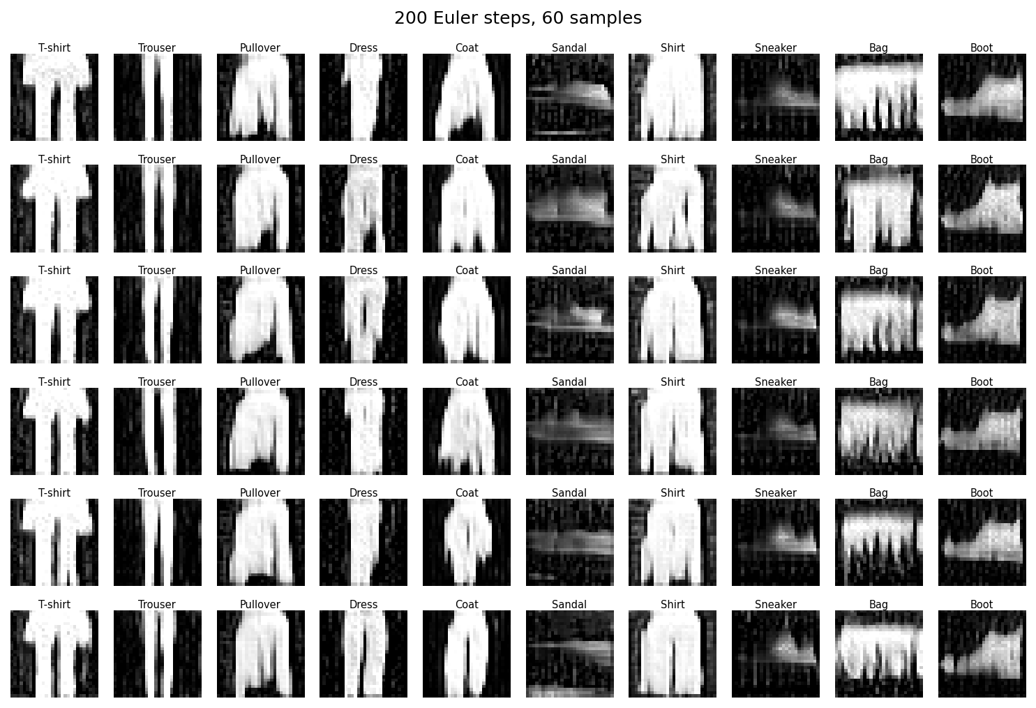
“Pantsiness” Reward

Originally, I was planning on setting up a reward for prompt-image alignment (prompt just being the class label for the type of clothing item). However, post-training had very little visible effect since CFG was already very effective at generating items with good alignment. So instead I tried to do the opposite, and see if you can post-train the model to “break” prompt-image alignment and always generate something that looks like one class: “pants” / Fashion-MNIST’s Trouser label. The reward is the frozen classifier’s log-probability for the Trouser class, ignoring the prompt.

In the sample grid, each generated class still retains characteristics of the guidance class, but is still somewhat able to fool the classifier into thinking it belongs to the Trouser class.

The training curve shows the Trouser reward increasing over the course of training:

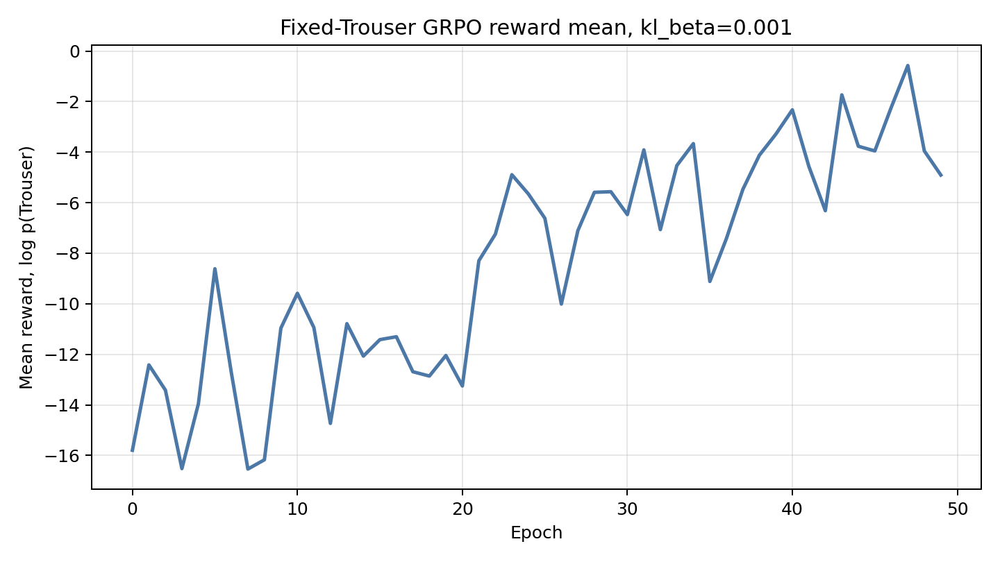
• Reward: fixed log p(Trouser | sample) under the Fashion classifier, ignoring the prompt.
• Training: 50 epochs, batch 4, $G=32$, num_inner=12, lr=1e-4, kl_beta=0.001, clip_eps=1.0, advantage_scale=20.0.
• Estimated compute: ~0.915 PFLOPs.
• Wall time: ~16.7 minutes.

JPEG Compressibility

We were able to reduce the JPEG bits per pixel (bpp) by roughly 20%.

This reward is more plausible than the previous one. The idea here is that we may want the model to produce images that are easier to compress. The reward is negative JPEG bits per pixel (bpp), so lower bpp gives a higher reward.

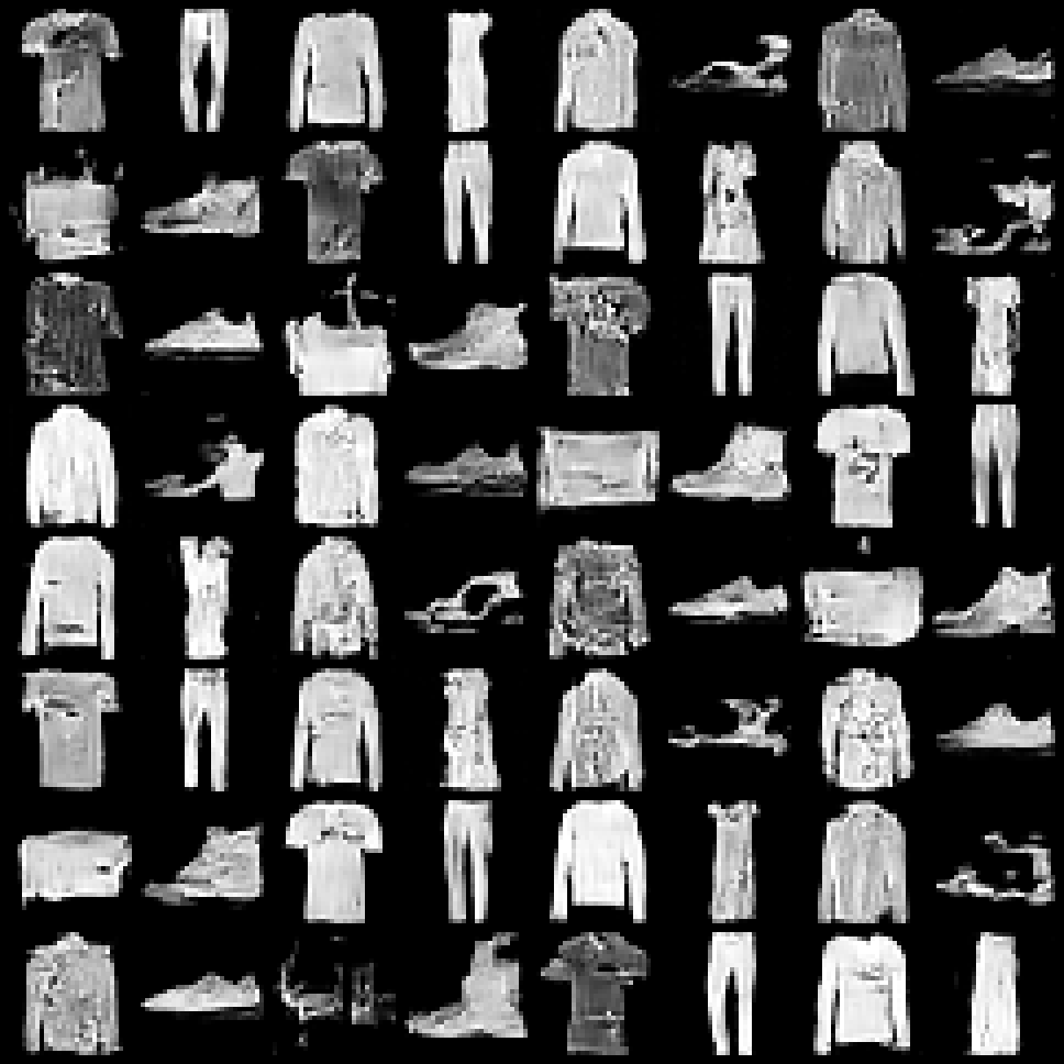
Original samples (before GRPO)

After training with JPEG bpp reward: 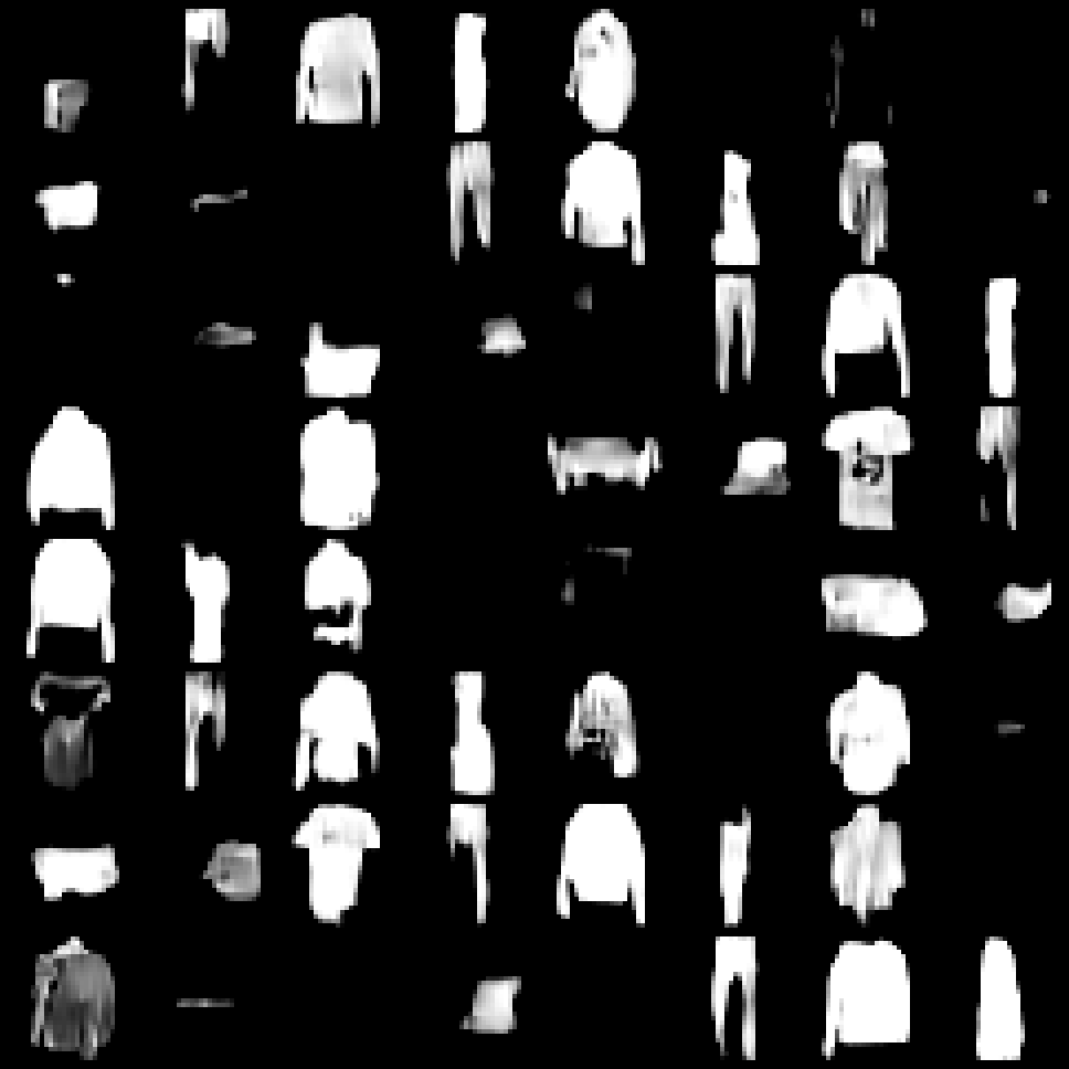The difference between shirts and pants is still visible, but quality suffered a lot. We could tweak the KL regularization strength (kl_beta) to prevent changing the distribution too much, if we wanted to avoid this.

• Reward: terminal black-box reward, reward(x) = -jpeg_bits_per_pixel(x).
• Training: 300 epochs, batch 4, $G=8$, num_inner=6, lr=2e-5, clip_eps=0.5, kl_beta=0.01, advantage_scale=5.0.
• Estimated compute: ~0.700 PFLOPs.
• Wall time: ~11.1 minutes.
• JPEG bpp: 6.2736 -> 4.9990, about a 20.3% reduction.
• PNG bpp: 5.3020 -> 2.6207.
• Classifier accuracy: 0.9531 -> 0.6094 (suffers as a result of loss of detail).

Code pointers:

• train_grpo.py
• rl/sde_sampler.py
• rl/grpo.py
• rl/reward.py
• rl/compression.py
• configs/experiment/fashion_grpo*.yaml
• configs/reward/fashion_*.yaml
• configs/rl_training/*.yaml
• experiments/jpeg_compression_grpo/experiment.md

Stage 3: CIFAR-10

CIFAR-10 is RGB, slightly higher resolution, and much more diverse (not just clothes). The U-Net is scaled up and training is run on a consumer GPU (4080 16GB VRAM) for much longer. It’s really hard to get an accurate idea of the quality of the generated images at such low resolution.

Data & Model

• Dataset: CIFAR-10, 60,000 total samples, 10 classes, 50,000 train / 10,000 test.
• Shape: 32x32 RGB.
• Model: class-conditional U-Net, RGB input, base 128, depth 3, bottleneck attention.
• Exact model size: 22,311,299 parameters for ClassCondUNet. For comparison, the unconditioned UNet with the same CIFAR config has 22,308,483 parameters.

The CIFAR model is the same basic U-Net family as the Fashion-MNIST model, but scaled substantially: input channels increase from 1 to 3, base_ch increases from 32 to 128, depth increases from 2 to 3, and bottleneck attention is enabled. Class conditioning is implemented by embedding the class label and adding that embedding to the timestep embedding. CFG uses an extra learned null class token, sampled during training according to training.p_uncond, so the same network can produce conditional and unconditional velocity predictions at sampling time.

Training Recipe

• 500 epochs, 97.5k steps, 24.96M training samples.
• Estimated compute: ~320 PFLOPs.
• Wall time: ~4.1–4.3 hours on RTX 4080.
• Peak GPU memory in TensorBoard: ~4.9GB.

Code pointers:

• configs/experiment/cifar10.yaml
• configs/experiment/cifar10_cfg.yaml
• configs/dataset/cifar10.yaml
• configs/model/unet_cifar.yaml
• configs/model/classcond_unet_cifar.yaml
• configs/metrics/fid_cifar10.yaml
• metrics.py

Reproduction details live in experiments/cifar10.md in the NanoFlow repository.

Stage 4: ImageNet-256

ImageNet-256 is much larger than previous datasets:

• 1000 classes
• 1.4M 256x256 RGB images
• Still used in some recent papers for benchmarking diffusion model performance (though mainly in some pixel diffusion models).

As a result, it was very challenging to stick with the original $100 training budget for the final run. We also wanted to avoid spending too much money and time on exploratory runs, so we had to be thoughtful about what runs we launched and how we chose to scale the model.

To try to offset the cost of training at higher resolution, we pre-processed the training dataset to generate a dataset of cached latents using SD VAE, generating [4, 32, 32] shaped latents for each image.

U-Net Baseline

For the initial training attempt, we re-used the same model architecture from Fashion-MNIST and CIFAR-10, just scaled up to ~89.8M parameters. Additionally, we moved from training on our own consumer desktop GPU to training on H100-SXM on RunPod.

Data & Model

• Dataset: ImageNet-256 SD-VAE latent cache.
• VAE: stabilityai/sd-vae-ft-ema.
• Model: ClassCondUNet in latent space.
• Model size: ~89.8M parameters.

Code/data pointers:

• docs/imagenet256_storage.md
• configs/dataset/imagenet256_latent_mmap.yaml
• configs/vae/sd_vae_ft_ema.yaml
• datasets.py
• vae.py

Training Recipe

• Config: 400 epochs, batch size 1024, bf16, EMA disabled.
• Training wall time from TensorBoard: about 16.5 H100-hours.
• Cost at USD $3.30/H100-hour: about USD $54.45.
• Approximate training compute: 16.4G train FLOPs/image × 1,281,167 train images × 400 epochs ≈ 8.4 EFLOPs.

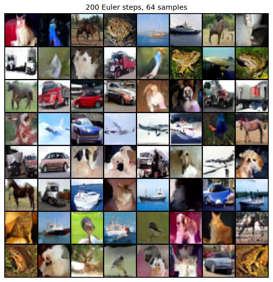
Diffusion Transformer

Clearly the image quality is not great for the U-Net model we trained, so even though the first model was in our budget we decided to explore ways to scale up the model.

Besides U-Net denoisers, Diffusion Transformers (DiTs) are another common architecture for training diffusion-style image generators, especially when scaling up the model. In order to keep costs manageable when trying a DiT, we tried several training-efficiency techniques, largely inspired by the paper Stretching Each Dollar: Diffusion Training from Scratch on a Micro-Budget:

• Deferred masking: mask out 75% of tokens after some initial DiT blocks (the patch mixer) during pre-training, then fine-tune with unmasked tokens to avoid train-test shift.
• Expert-choice MoE: increase model capacity without a large increase in compute FLOPs.
• Layerwise scaling: make transformer layers wider in deeper layers. This pairs well with deferred masking, since the early layers are cheaper per token where we have the most tokens.

Additionally, we added some simple training optimizations to our training code:

• PT2 compile
• bf16 automatic mixed precision
• packed MoE

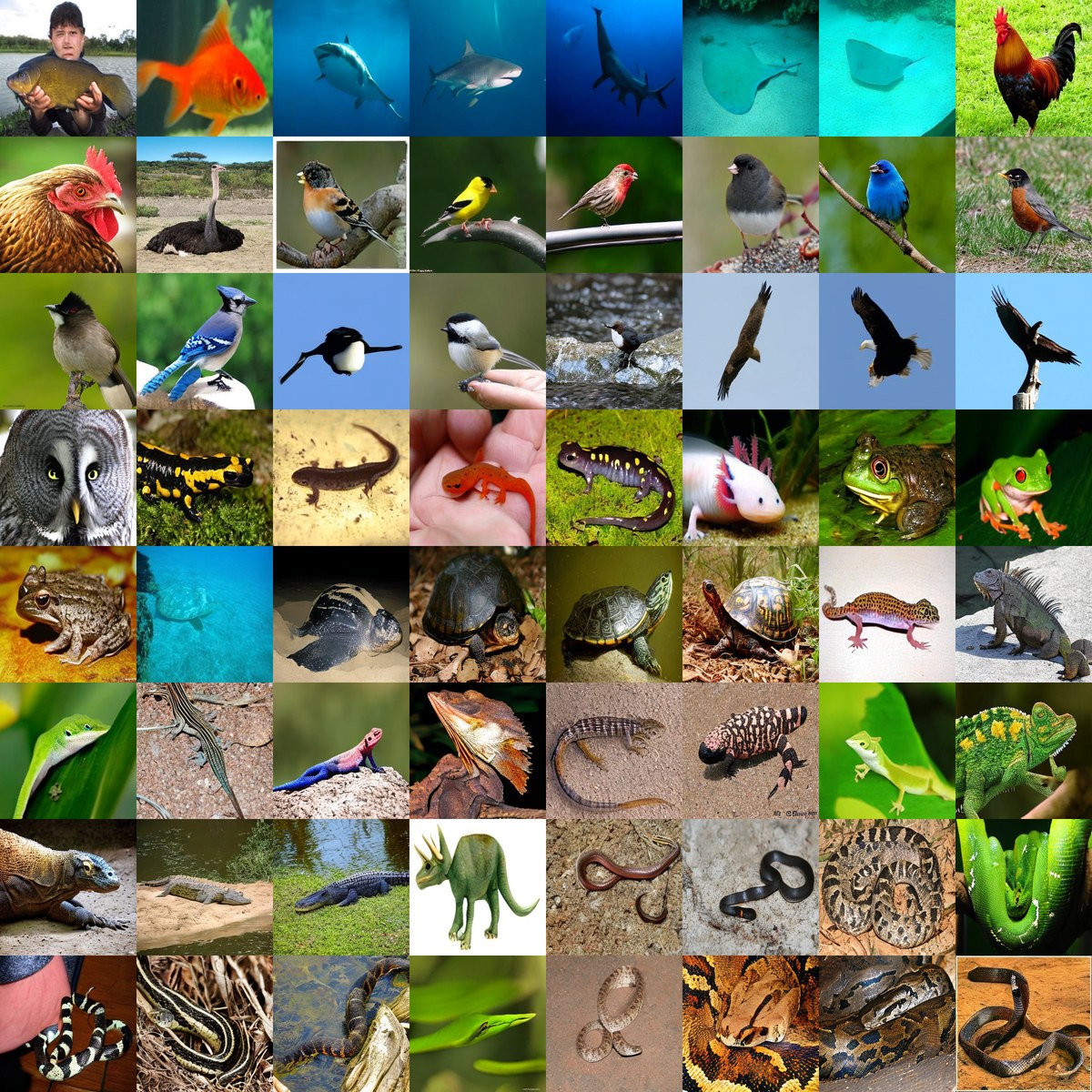
The end result is much better quality, though the quality is still very far from comparable papers training cheap pixel-space diffusion models on ImageNet-256. For instance, both PixNerd and SiD2 have much higher training cost, although they achieve very low FID:

• PixNerd-XL/16: ~480 reported GPU-hours, ~$1.6k.
• SiD2-small: FLOP-derived lower bound of ~470 H100-equivalent hours, ~$1.6k.
• SiD2 flop-heavy: FLOP-derived lower bound of ~1,800 H100-equivalent hours, ~$5.9k. The lower-compute 256-to-512 finetune point is ~640 H100-equivalent hours, or ~$2.1k.

So it’s more common to train an ImageNet model with hundreds to thousands of GPU-equivalent hours (not the ~64 H100 GPU hours we trained on). Even so, scaling up the model more than doubled the original training budget for the run: $210.45 versus the initial $100 target.

Additionally, we would have liked to run some FID evals just to get an objective sense of the model performance, but our rough estimate on 30k/50k sample generation alone is on the order of 5.7/9.5 EFLOPs of forward sampling before VAE decode, which is actually similar cost to our U-Net training run for single eval. As a result we decided to forego doing FID comparison.

Data & Model

• Dataset: ImageNet-256 SD-VAE latent mmap cache.
• Model: H1024 D20 E16 c2 moew0.5 deferred-masking DiT.
• Total parameters: 695.1M.
• Token-average active parameters: 314.0M.
• Final-best model compute estimate: 240 masked epochs × 1,281,167 images × 86.72G train FLOPs/image + 40 unmasked epochs × 1,281,167 images × 284.86G train FLOPs/image ≈ 41.3 EFLOPs.
• Runtime: 63.7714 H100-hours.
• Cost at USD $3.30/hr: USD $210.45.

Budget breakdown & wall time:

• Masked pretrain: 240 total epochs at 14.45G MACs/image, or ~86.72G train FLOPs/image.
  • Initial masked pretrain: 13h36m36s, 13.6100 H100-hours, $44.91.
  • Masked continuation: 28h13m47s, 28.2297 H100-hours, $93.16.
• Low-LR unmasked fine tuning: 40 epochs at 47.48G MACs/image, or ~284.86G train FLOPs/image.
  • 21h55m54s, 21.9317 H100-hours, $72.37.
• Total final-best model: 63h46m17s, 63.7714 H100-hours, $210.45.

Code pointers

• docs/runpod_imagenet256_dit_chain.md
• docs/imagenet_eval.md
• cloud/runpod/imagenet256-dit-h1024-d20-training-chain.yaml
• configs/experiment/imagenet256_latent_dit_m2_moe_layerwise_h1024_d20_e16_c2_moew05_masked80.yaml
• configs/experiment/imagenet256_latent_dit_m2_moe_layerwise_h1024_d20_e16_c2_moew05_unmasked20.yaml
• configs/model/classcond_deferred_dit_imagenet256_latent_m2_moe_layerwise_h1024_d20_e16_c2_moew05.yaml
• models_dit.py
• eval_imagenet.py

Reproduction details live in experiments/imagenet256.md in the NanoFlow repository.

Conclusion

This was great learning on how viable it is to explore from-scratch training for flow matching models on a hobbyist budget. We ended up going from training ~539 GFLOPs to ~41 EFLOPs on increasingly non-trivial datasets. It’s hard, but not impossible to train a decent looking ImageNet-256 model (if you don’t look too hard at your generated images!), but unless you’re willing to shell out thousands of dollars for training it’s not something you can experiment too much with. Probably it would have been a better choice to try ImageNet-64 first, as that would have been a bit easier to try.

We also got some hands-on experience with post-training on image diffusion models. Post-training was more complicated than pre-training, due to managing both rollouts and training, as well as many knobs to tune. There is also a lot of flexibility in terms of what rewards to optimize for.

This project felt very different from my industry experience training ML models. Typically spending even hundreds of hours of GPU time is not a big deal even for exploratory runs or evals, but running hobbyist experiments on your own dime changes a lot about how you think about compute. I was a lot more conscious of estimating the E2E training cost before launching the run, and more pre-emptive about searching for ways to reduce the cost of the E2E training run.