Diffusion Model Probability Paths Visualized

Probability Paths

Diffusion models iteratively map noise to data. There’s many approaches to diffusion models, but largely they share a similar approach (DDPM, NCSN, SGM, FGM) for Gaussian probability paths:

sample a data point
based on a selected noising process, sample a noised point (no need to directly simulate each step for Gaussian processes)
also based on the noising process and the data point, calculate which direction to go to follow a corresponding denoising process (either in terms of a vector field, score function, or applying ELBO to variational Markov chain)

The choice of probability paths makes a meaningful difference to the quality of the trained models.

Variance Exploding path (VE) introduced in NCSN ¹
Variance Preserving path (VP) ², as well as the sub-variance preserving path ³.
Conditional Optimal transport (CondOT) path introduced in FGM⁴.

To motivate why the probability path matters for training diffusion models, consider the flow and score matching losses.

For flow matching:

\[\mathcal{L}_\text{CFM}(\theta) = \mathbf{E}_{t \sim \text{Unif}, z \sim p_\text{data}, x \sim p_t(\cdot | z)} \| u_t^\theta (x) - u_t^\text{target} (x | z) \|^2\]

or in the case of flow matching (SDE):

\[\mathcal{L}_\text{CSM}(\theta) = \mathbf{E}_{t \sim \text{Unif}, z \sim p_\text{data}, x \sim p_t(\cdot | z)} \| s_t^\theta (x) - \nabla \log p_t (x | z) \|^2\]

In both cases the target, either $u_t^\text{target}(x | z)$ or $\nabla \log p_t(x | z)$ are determined by the probability path. Additionally the sampling $x \sim p_t(\cdot | z)$ is determined by choice of probability path.

Intuition about the forward process

Although it’s the probability path that we care about for training, it’s helpful to look at what is the “noising” process that is used to generate training samples. The forward process dictates which “noised” data points are used to learn the probability vector field or score function.

The probability path and SDE are related via the Fokker-Planck equation, so for the rest of this section we proceed by simulating the corresponding forward SDE.

Here is one example simulated SDE path corresponding to each probability path: Example SDE forward path

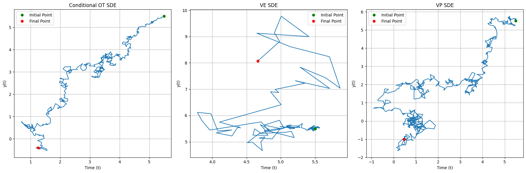
Observe that both CondOT and VP paths tend to walk towards the origin, while the VE path looks like a random walk.

We can confirm this by simulating more samples from the SDE and estimating the distribution over time:

For VE, the plot doesn’t show any non-zero probability since for the first 300 or so timesteps it’s just an impulse (which doesn’t show on the low spatial resolution plot).

Plotting the stats from simulating the forward SDE: SDE Stats Perturbation Kernel

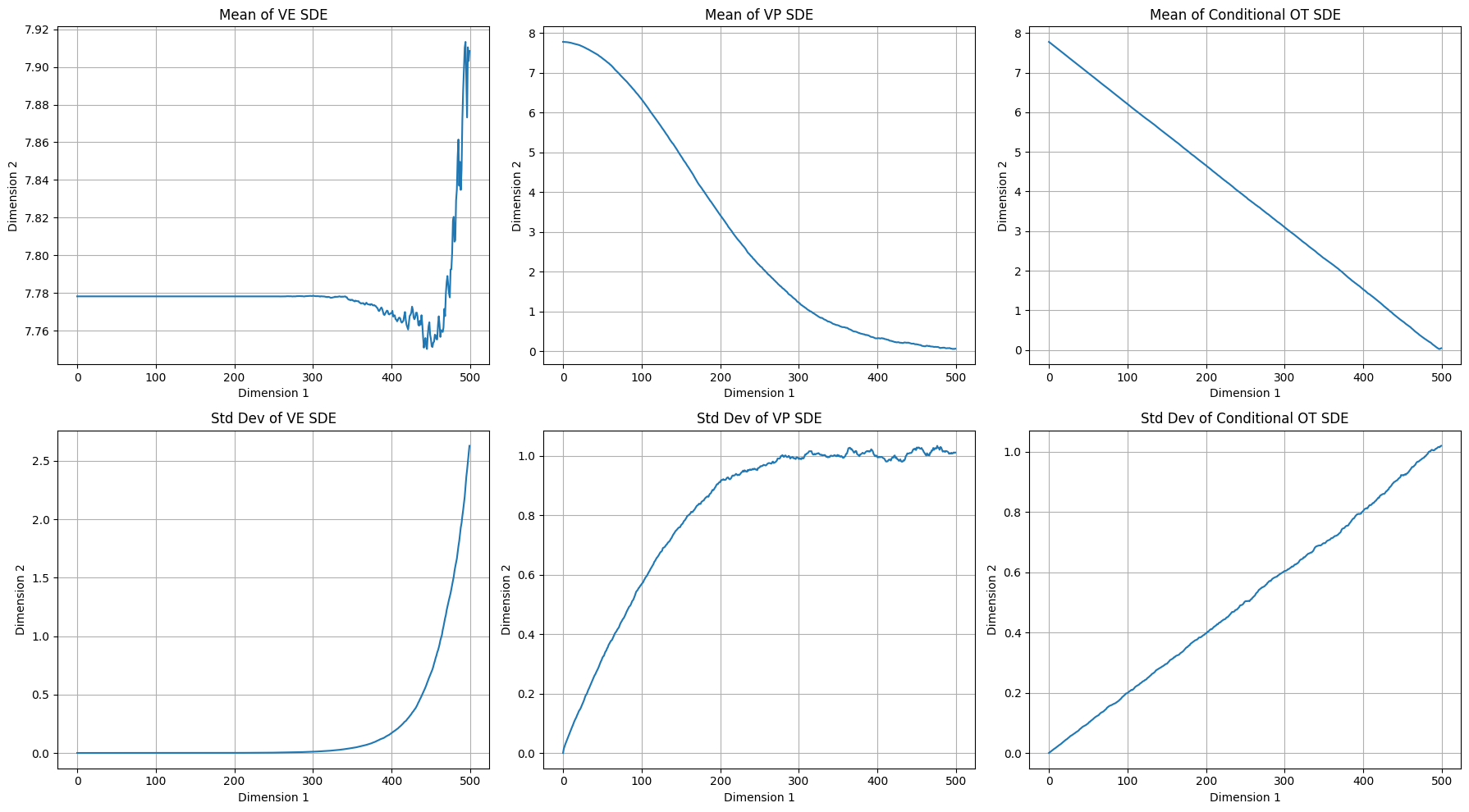
Takeaways:

CondOT is designed to linearly interpolate between dirac delta centered at $z$ and standard normal. Sampling $t \sim \text{Uniform}$ will give us points that are uniformly between $z$ and $0$, and also uniform in terms of variance.
If we sample uniformly for VE according to time, we will get samples with very low variance on average. In NCSN the loss is weighted to up-weight samples with higher variance to overcome this (though NCSN the method doesn’t do sampling, it’s just the weighted sum).
VP spends most of it’s time close to $p_\text{init}$ or $p_\text{data}$.

Probability Flows

Here’s what the conditional solutions look like for each probability path (again same fixed datapoint $z$ for each).

VE vector field is time invariant, flowing direclty towards $z$.
For VE it is not the case that $p_0 \sim \mathcal{N}(0, I)$, as the variance at $p_0$ is not close to 1 for the standard choice of hyperparams.
VP path does not flow straight, while other probability paths do. This complicates training and sampling numerically.
- Initially only the constant drift term applies for VP, then there is probability flow towards $z$ as $t \rightarrow 1$.
CondOT flows straight, with vector field pulling more strongly towards $z$ as $t \rightarrow 1$.

Equations Reference

Here we use the convention that $p_s \sim p_\text{data}$ for $s = 0$ and $p_t \sim p_\text{data}$ for $t = 0$.

Name	Variance Exploding (VE) ⁵	Variance Preserving (VP) ⁶	CondOT ⁷
Forward Conditional Probability path (i.e. perturbation kernel)	$p_s(x_s \| z) = \mathcal{N}(x_s \| z, \sigma_{s}^2 \mathbf{I})$	$p_s(x_s \| z) = \mathcal{N}(x_s \| \alpha_{s} z, (1 - \alpha_{s}^2) \mathbf{I})$	$p_s(x_s \| z) = \mathcal{N}(x_s \| (1 - s) z, [\sigma_\text{min} + (1 - \sigma_\text{min}) s]^2 \mathbf{I})$
Reverse Conditional Probability Path	$p_t(x_t \| z) = \mathcal{N}(x_t \| z, \sigma_{1 - t}^2 \mathbf{I})$	$p_t(x_t \| z) = \mathcal{N}(x_t \| \alpha_{1 - t} z, (1 - \alpha_{1 - t}^2) \mathbf{I})$	$p_t(x_t \| z) = \mathcal{N}(x_t \| t z, [1 - (1 - \sigma_\text{min}) t]^2 \mathbf{I}$)
Forward SDE	$dX_s = \sqrt{\frac{d(\sigma_s^2)}{ds}} dW_s$	$dX_s = -\frac{1}{2} \beta_s X_s ds + \sqrt{\beta_s} dW_s$	$dX_s = [(\frac{\alpha_s (1 - \sigma_\text{min}) - \frac{\sigma_s^2}{2}}{\alpha_s^2})(X_s - (1 - s)z) - z] ds + \sigma_s dW_s$
Reverse SDE	$dX_t = \lbrack (\sigma_\text{min} \ln \frac{\sigma_\text{max}}{\sigma_\text{min}} + \frac{\sigma_t^2}{2 (\frac{\sigma_\text{max}}{\sigma_\text{min}})^{1 - t}}) (z - X_t) \rbrack dt + \sigma_t dW_t$	$dX_t = \frac{1}{2 (1 - \alpha_{1 - t}^2)} \lbrack - \dot{\alpha}_{1 - t} (z - \alpha_{1 - t} X_t) + \frac{\sigma_t^2}{2} (\alpha_{1 - t} z - X_t) \rbrack dt + \sigma_t dW_t$	$dX_t = \lbrack \frac{z - (1 - \sigma_\text{min}) X_t}{\alpha_{1 - t}} + \frac{\sigma_t^2 (t z - X_t)}{2 \alpha_{1 - t}^2} \rbrack dt + \sigma_t dW_t$
Conditional Vector Field	$u_t(x \| z) = \sigma_\text{min} \ln \frac{\sigma_\text{max}}{\sigma_\text{min}}(z - x)$	$u_t(x \| z) = -\frac{\dot{\alpha}_{1 - t}}{1 - \alpha_{1 - t}^2} (z - \alpha_{1 - t} x)$	$u_t(x \| z) = \frac{z - (1 - \sigma_\text{min}) x }{1 - (1 - \sigma_\text{min})t}$
Conditional Flow	$\psi_t({x \| z}) = \sigma_\text{min} (\frac{\sigma_\text{max}}{\sigma_\text{min}})^{1 - t} x + z$	$\psi_t(x \| z) = \sqrt{1 - \alpha_{1 - t}^2} x + \alpha_{1 - t} z$	$\psi_t(x \| z) = x + t (z - (1 - \sigma_\text{min}) x)$

Appendix

Colab: Gaussian Probability Paths in Diffusion Models

Song and Ermon 2020 ↩
Ho et al. 2020 ↩
Song et al. 2021 ↩
Lipman et al. 2023 ↩
For $\sigma_s = \sigma_\text{min}(\frac{\sigma_\text{max}}{\sigma_\text{min}})^s$ ↩
For $\alpha_t = e^{- \frac{1}{2} T(t)}, \quad T(t) = \int_0^t \beta_s ds, \quad \beta_t = \bar{\beta}_\text{min} + t (\bar{\beta}_\text{max} - \bar{\beta}_\text{min})$ ↩
For $\alpha_t = \sigma_\text{min} + (1 - \sigma_\text{min}) t$ ↩

Name	Variance Exploding (VE) ⁵	Variance Preserving (VP) ⁶	CondOT ⁷
Forward Conditional Probability path (i.e. perturbation kernel)	$p_s(x_s \| z) = \mathcal{N}(x_s \| z, \sigma_{s}^2 \mathbf{I})$	$p_s(x_s \| z) = \mathcal{N}(x_s \| \alpha_{s} z, (1 - \alpha_{s}^2) \mathbf{I})$	$p_s(x_s \| z) = \mathcal{N}(x_s \| (1 - s) z, [\sigma_\text{min} + (1 - \sigma_\text{min}) s]^2 \mathbf{I})$
Reverse Conditional Probability Path	$p_t(x_t \| z) = \mathcal{N}(x_t \| z, \sigma_{1 - t}^2 \mathbf{I})$	$p_t(x_t \| z) = \mathcal{N}(x_t \| \alpha_{1 - t} z, (1 - \alpha_{1 - t}^2) \mathbf{I})$	$p_t(x_t \| z) = \mathcal{N}(x_t \| t z, [1 - (1 - \sigma_\text{min}) t]^2 \mathbf{I}$)
Forward SDE	$dX_s = \sqrt{\frac{d(\sigma_s^2)}{ds}} dW_s$	$dX_s = -\frac{1}{2} \beta_s X_s ds + \sqrt{\beta_s} dW_s$	$dX_s = [(\frac{\alpha_s (1 - \sigma_\text{min}) - \frac{\sigma_s^2}{2}}{\alpha_s^2})(X_s - (1 - s)z) - z] ds + \sigma_s dW_s$
Reverse SDE	\(dX_t = \lbrack (\sigma_\text{min} \ln \frac{\sigma_\text{max}}{\sigma_\text{min}} + \frac{\sigma_t^2}{2 (\frac{\sigma_\text{max}}{\sigma_\text{min}})^{1 - t}}) (z - X_t) \rbrack dt + \sigma_t dW_t\)	\(dX_t = \frac{1}{2 (1 - \alpha_{1 - t}^2)} \lbrack - \dot{\alpha}_{1 - t} (z - \alpha_{1 - t} X_t) + \frac{\sigma_t^2}{2} (\alpha_{1 - t} z - X_t) \rbrack dt + \sigma_t dW_t\)	\(dX_t = \lbrack \frac{z - (1 - \sigma_\text{min}) X_t}{\alpha_{1 - t}} + \frac{\sigma_t^2 (t z - X_t)}{2 \alpha_{1 - t}^2} \rbrack dt + \sigma_t dW_t\)
Conditional Vector Field	$u_t(x \| z) = \sigma_\text{min} \ln \frac{\sigma_\text{max}}{\sigma_\text{min}}(z - x)$	\(u_t(x \| z) = -\frac{\dot{\alpha}_{1 - t}}{1 - \alpha_{1 - t}^2} (z - \alpha_{1 - t} x)\)	$u_t(x \| z) = \frac{z - (1 - \sigma_\text{min}) x }{1 - (1 - \sigma_\text{min})t}$
Conditional Flow	\(\psi_t({x \| z}) = \sigma_\text{min} (\frac{\sigma_\text{max}}{\sigma_\text{min}})^{1 - t} x + z\)	\(\psi_t(x \| z) = \sqrt{1 - \alpha_{1 - t}^2} x + \alpha_{1 - t} z\)	\(\psi_t(x \| z) = x + t (z - (1 - \sigma_\text{min}) x)\)