Variational Auto-Encoders(VAE) are an extension of Auto-Encoders(AE) which allow a probabilistic representation of the latent space. Rather than learning a deterministic latent representation of the data, VAE instead learns a distribution over the latent space. This blog post is intended as a quick and dirty introduction to understanding and working with VAE. We will not go into too much detail on the math or new developments and applications of VAE, instead focusing on showing code examples applied to MNIST. First we’ll give a brief overview and some examples of AE and then introduce VAE.

Auto-Encoder Overview

Auto-Encoders(AE) are a type of unsupervised model that aims to learn a latent representation of the data. An advantage to learning a latent representation might be to leverage unlabeled data to generate features for some other task, or to decrease the dimensionality of the features, as the latent space is usually chosen to be lower dimensional than the input space. In some sense, AE can be thought of as similar to Prinicipal Component Analysis(PCA), a method which also seeks to learn a latent representation. Actually, if we restrict our encoder and decoder networks to be linear(i.e. no activation function, fully connected layers), then the optimal solution would be the same as PCA!

Autoencoder

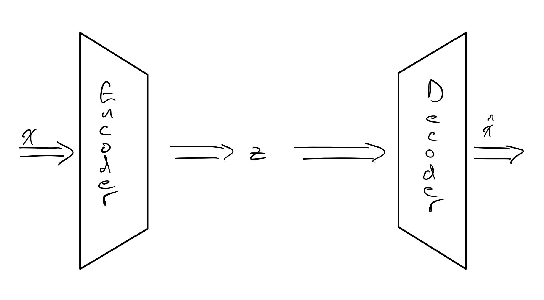
AE are composed of two component networks: the encoder and the decoder. The encoder maps the input space to the latent space, and the decoder does the inverse of this and maps the latent space to the input space. Although the decoder inverts the encoder, it does not need to have the same architecture. For example, our input network could be convolutional, but we could choose any architecture, such as fully connected, for our decoder. The loss used to train the network is some form of reconstruction loss, which evaluates the reconstructed $\mathbf{\hat{x}}$ against $\mathbf{x}$, e.g. Mean-Square Error(MSE).

The encoder $f$ gives us $\mathbf{z} = f(\mathbf{x})$ and the decoder $g$ gives us $\mathbf{\hat{x}} = g(\mathbf{z})$. What can we use the latent features $\mathbf{z}$ and the reconstruction $\mathbf{\hat{x}}$ for?

The latent feature $\mathbf{z}$ could be used for any number of things. Auto-Encoders could help us generate low dimensional representations of our data, which could be useful for visualization. While we could fit a PCA model on the raw image data, this might not be a great idea since image data is highly non-linear. Here is an example of PCA run on the latent features $\mathbf{z}$ output from the encoder.

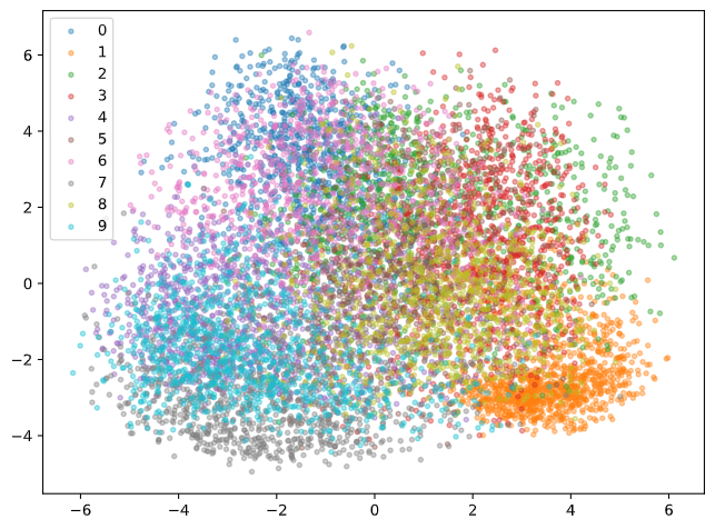
Example of 2D PCA Representation of Latent Features of MNIST.

The numbers look a bit mixed up still, but a few labels such as 1 and 9 form some more coherent clusters. Keep in mind also, this only takes the first two principal components, i.e. good separation of all classes is incredibly hard to achieve in just 2 dimensions.

Looking at the reconstruction $\mathbf{\hat{x}}$ is important for qualitatively assessing the performance of an Auto-Encoder. Here we can see the original and reconstructed images for the MNIST Auto-Encoder.

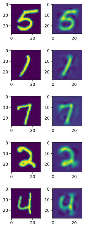
Original(left) and reconstructed(right) MNIST images.

In addition to assessing the model quality, the reconstruction $\hat{\mathbf{x}}$ can also be used for collaborative recommendation systems and anomaly detection. For collaborative recommendation systems, such as in [1], the model is trained to encode the sparse input $\mathbf{x}$ into a latent space. Then the reconstructed $\mathbf{\hat{x}}$ is encouraged by a specific loss function, Masked Mean-Square Error(MMSE), to be dense. The dense $\mathbf{\hat{x}}$ can be used to predict what products a user will like. In the case of anomaly detection, $\mathbf{\hat{x}}$ and $\mathbf{x}$ can be used to calculate the reconstruction error. Samples with high reconstruction error may be deemed to be anomalous, as the model is more likely to perform better reconstruction on samples close to the manifold of training samples(the non-anomalous data).

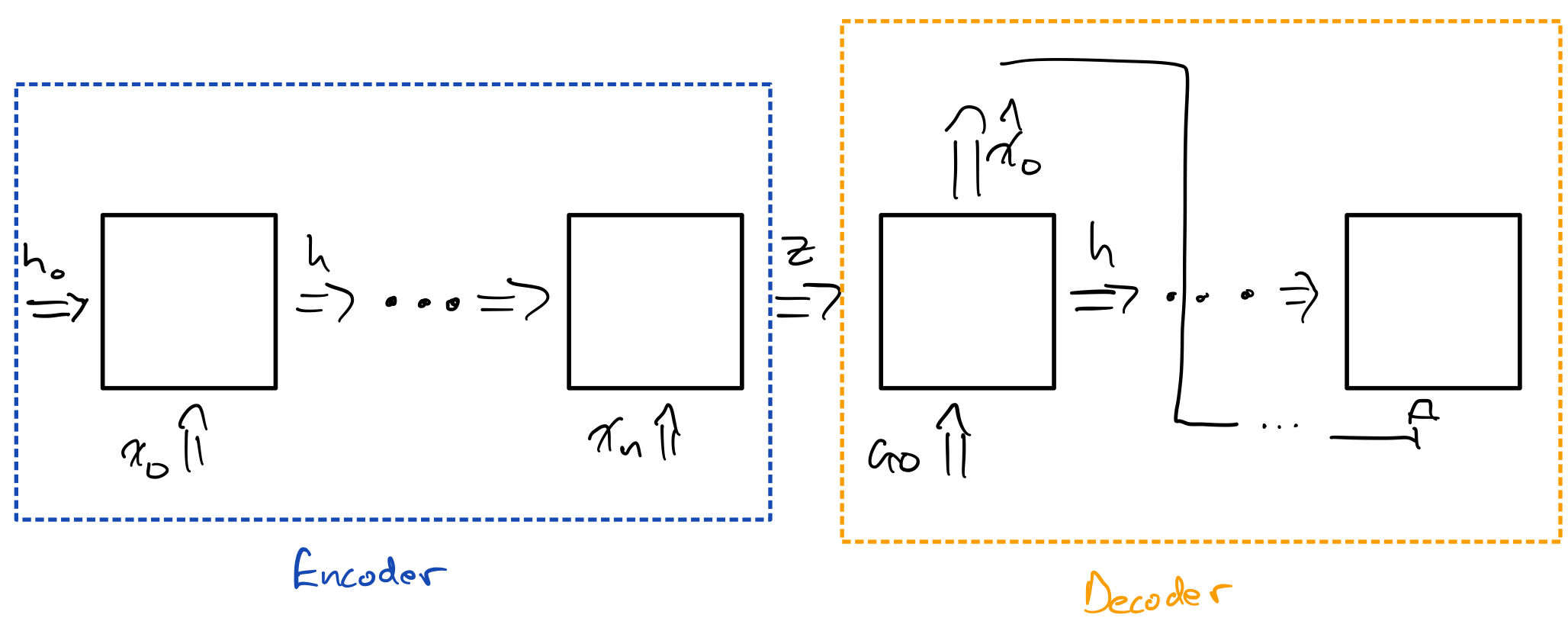
Before moving on, let’s talk about how flexible AE are and how they can be used in various contexts. The architecture for AE is very general, and we have a lot of freedom to choose our encoder and decoder structure based on the task. For example, although the above 2D PCA figure and the reconstruction example are from a fully connected AE, we could easily modify the network to use convolutional layers. Another example of the flexibility of AE is how we can use recurrent networks for encoder and/or decoder. In fact, if you’ve ever used a sequence to sequence model, such as in a translation task, you’ve seen what is essentially an AE for sequences. The encoder in this case is a RNN, which takes in a sequence. The decoder is also an RNN, which feeds it’s output back into itself. The latent state $\mathbf{z}$ is the hidden state that gets passed from the last encoding RNN cell to the first decoding RNN cell. $\mathbf{z}$ should contain all the information needed to reconstruct the sequence.

Now that we’ve reviewed some basics about AE and how they are used, let’s introduce Variational Auto-Encoders.

Variational Auto-Encoder Overview

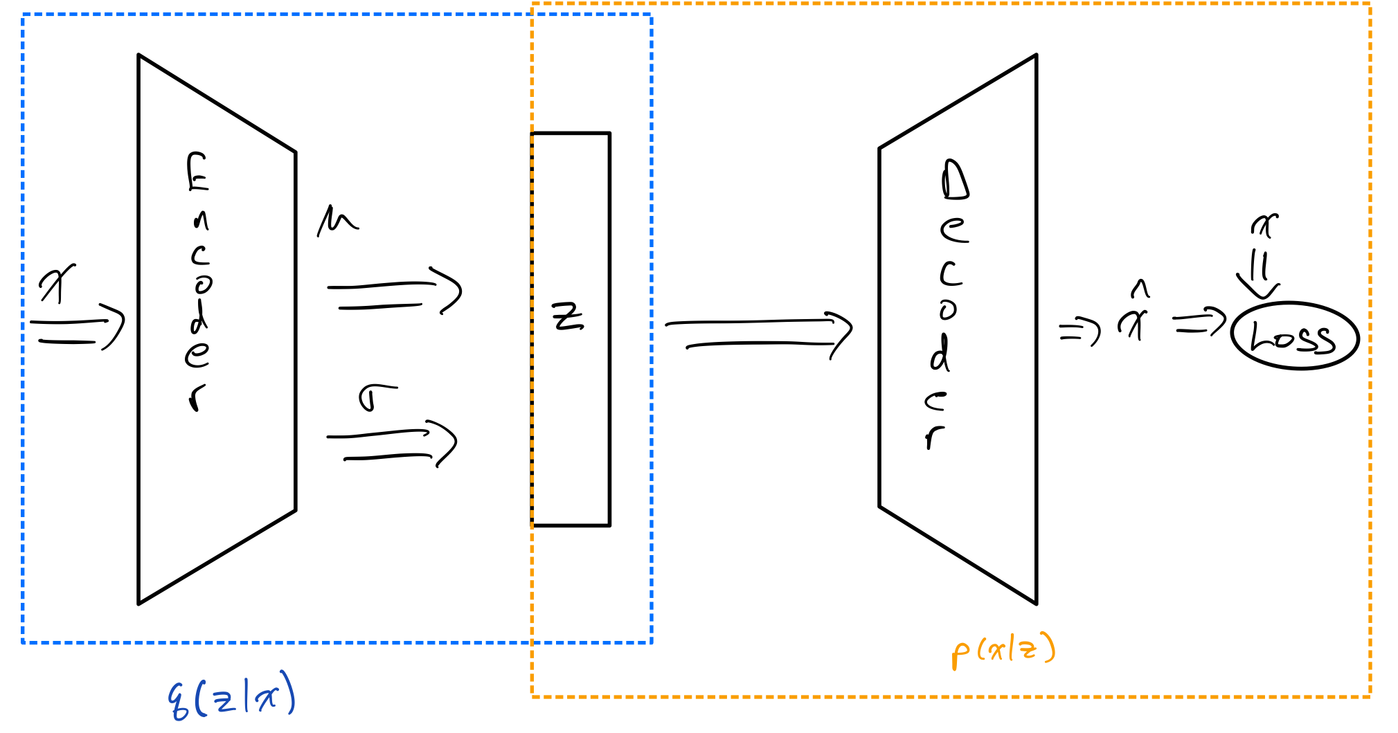
Variational Auto-Encoder(VAE) was introduced in the seminal paper by Kingma and Welling [2] as a way to apply Stochastic Variational Inference(SVI) to training a probabilistic Auto-Encoder. The idea behind VAE is still much the same as the AE case. We will still encode the data using an encoder network, and reconstruct the input from the latent space using a decoder network. However, the key difference is that the latent features that the encoder maps to are no longer deterministic. In other words, instead of learning a deterministic function $\mathbf{x} \rightarrow f(\mathbf{x})$, our goal is to learn a conditional distribution $p(\mathbf{z}|\mathbf{x})$.

VAE

Unfortunately, in the general case finding the posterior $p(\mathbf{z}|\mathbf{x})$ is not tractable. The term variational describes the fact that we will approximate $p(\mathbf{z}|\mathbf{x})$ using a variational distribution $q(\mathbf{z}|\mathbf{x})$, which comes from a simpler family of distributions. Often in the case of VAE, the family of distributions that $q$ is constrained to is the class of multivariate normal distributions with diagonal variance.

Why might we want to use VAE instead of regular AE? Well, for one the model is Bayesian. The posterior $p(\mathbf{z}|\mathbf{x})$ is calculated as:

\[p(\mathbf{z}|\mathbf{x}) = \frac{p(\mathbf{x}|\mathbf{z}) p(\mathbf{z})}{\int_{\mathbb{R}^n} p(\mathbf{x}|\mathbf{z}) p(\mathbf{z}) d\mathbf{z}}\]

As a result, we have additional control over how our model learns the latent representation. Also, as we will see in the next section, one part of the loss is a regularization term that penalizes learning distributions far from the prior. We can control the amount of regularization by weighting the reconstruction loss vs the regularization loss from deviating from the prior. Such an approach is known as $\beta$-VAE, for the hyperparameter that determines the weighting, $\beta$. Finally, VAE can be used as a generative model. By sampling from the prior distribution and passing the sampled latent space samples through the decoder, we can sample from $p(\mathbf{x})$.

For a more in-depth tutorial and overview of VAE, see [3].

VAE Loss and Training

The goal of training VAE is to simultaneously optimize the encoder to learn a good approximation $q(\mathbf{z}|\mathbf{x})$ to $p(\mathbf{z}|\mathbf{x})$ and at same time learn how to reconstruct $\mathbf{x}$ from the latent features. The decoder will determine our likelihood distribution $p(\mathbf{x}|\mathbf{z})$.

The way to determine whether $q(\mathbf{z}|\mathbf{x})$ is a good approximation of $p(\mathbf{z}|\mathbf{x})$ is to use the Kullback-Leibler Divergence(KLD). The KLD from probability measures $Q$ to $P$ is written as $D_{KL}(P||Q)$. KLD is asymmetric, meaning $D_{KL}(P||Q) = D_{KL}(Q||P)$ is not in general true. In the general case, KLD is defined as:

\[D_{KL}(P||Q) = \int_{\Omega} log(\frac{dP}{dQ}) dP\]

for $P$, $Q$ measures on $\Omega$ and $P$ absolutely continuous w.r.t $Q$.

The interpretation of KLD is that is that $D_{KL}(P||Q)$ describes the amount of information lost when using $Q$ to approximate $P$. So using KLD can give us a way of quantifying how close $q(\mathbf{z}|\mathbf{x})$ is to $p(\mathbf{z}|\mathbf{x})$. We’ll be using KLD as the loss of the network, seeking to minimize:

\[\begin{aligned} &\min_{\theta, \phi} D_{KL}(q_\phi(\mathbf{z}|\mathbf{x})||p(\mathbf{z}|\mathbf{x})) \\ &= \min_{\theta, \phi} \int_{\mathbb{R}^n} q_\phi (\mathbf{z}|\mathbf{x}) \log \frac{q_\phi (\mathbf{z}|\mathbf{x})}{p(\mathbf{z}|\mathbf{x})} d\mathbf{z} \\ &= \min_{\theta, \phi} \int_{\mathbb{R}^n} q_\phi (\mathbf{z}|\mathbf{x}) \log \frac{q_\phi (\mathbf{z}|\mathbf{x}) p(x)}{p(\mathbf{z}, \mathbf{x})} d\mathbf{z} \\ &= \min_{\theta, \phi} \int_{\mathbb{R}^n} q_\phi(\mathbf{\mathbf{z}}|\mathbf{\mathbf{x}}) (\log \frac{q_\phi(\mathbf{\mathbf{z}}|\mathbf{\mathbf{x}})}{p(\mathbf{\mathbf{z}}, \mathbf{\mathbf{x}})} + \log p(\mathbf{\mathbf{z}})) d\mathbf{\mathbf{z}} \\ &= \min_{\theta, \phi} \int_{\mathbb{R}^n} q_\phi(\mathbf{z}|\mathbf{x}) \log \frac{q_\phi(\mathbf{z}|\mathbf{x})}{p(\mathbf{z}, \mathbf{x})} d\mathbf{z} + \int_{\mathbb{R}^n} q_\phi(\mathbf{z}|\mathbf{x}) \log p(\mathbf{x}) d\mathbf{z} \\ &= \log p(\mathbf{x}) + \min_{\theta, \phi} \int_{\mathbb{R}^n} q_\phi(\mathbf{z}|\mathbf{x}) \log \frac{q_\phi(\mathbf{z}|\mathbf{x})}{p(\mathbf{z}, \mathbf{x})} d\mathbf{z} \\ &= \log p(\mathbf{x}) + \min_{\theta, \phi} E_{Q}[\log \frac{q_\phi(\mathbf{z}|\mathbf{x})}{p(\mathbf{z}, \mathbf{x})}] \end{aligned}\]

where $\phi$ are the parameters of the encoder and $\theta$ are the parameters of the decoder. $E_Q$ is the expectation w.r.t the measure defined by the distribution $q(\mathbf{z}|\mathbf{x})$. Note that although the expression does not contain $\theta$ at the moment, it will appear once $p_\theta(\mathbf{x}|\mathbf{z})$ appears. In the last step, $p(\mathbf{x})$ in the sum does not depend on either parameter $\theta$, $\phi$ so we can safely ignore it.

\[\begin{aligned} &\min_{\theta, \phi} E_{Q}[\log \frac{q_\phi(\mathbf{\mathbf{z}}|\mathbf{x})}{p(\mathbf{z}, \mathbf{x})}] \\ &= \min_{\theta, \phi} E_{Q}[\log \frac{q_\phi(\mathbf{z}|\mathbf{x})}{p_\theta(\mathbf{x}|\mathbf{z}) p(\mathbf{z})}] \\ &= \min_{\theta, \phi} - E_{Q}[\log p_\theta(\mathbf{x}|\mathbf{z}) + \log \frac{p(\mathbf{z})}{q_\phi(\mathbf{z}|\mathbf{x})}] \\ &= \min_{\theta, \phi} - E_{Q}[\log p_\theta(\mathbf{x}|\mathbf{z})] + D_{KL}(q_\phi(\mathbf{z}|\mathbf{x})||p(\mathbf{z})) \\ &= \min_{\theta, \phi} - \mathcal{L_{\theta, \phi}}(Q) \end{aligned}\]

Where $\mathcal{L_{\theta, \phi}}(Q) = E_{Q}[\log p_\theta(\mathbf{x}|\mathbf{z})] - D_{KL}(q_\phi(\mathbf{z}|\mathbf{x})||p(\mathbf{z}))$ is the Evidence Lower Bound. The naming for ELBO is justified as it is the lower bound of $\log p(\mathbf{x})$, the log evidence:

\[\log p(\mathbf{x}) = D_{KL}(q_\phi(\mathbf{z}|\mathbf{x})||p(\mathbf{z}|\mathbf{x})) + \mathcal{L_{\theta, \phi}}(Q)\]

assuming $D_{KL}(q_\phi(\mathbf{z}|\mathbf{x})||p(\mathbf{z}|\mathbf{x})) \geq 0$, which follows from Gibb’s inequality. To summarize, the loss in VAE training is the negative ELBO loss, and the ELBO loss is composed of two parts: the reconstruction loss and KLD from the prior to the variational conditional distribution.

Now that we understand the components of the loss, we can see that there are three distributions that need to be determined to calculate the loss: the likelihood $p_\phi(\mathbf{x}|\mathbf{z})$, the prior $p(\mathbf{x})$, and the variational posterior $q(\mathbf{z}|\mathbf{x})$. We’ve already alluded to the fact that the encoder network determines $q_\phi(\mathbf{z}|\mathbf{x})$ and the decoder network determines $p_\theta(\mathbf{x}|\mathbf{z})$. For $p(\mathbf{x})$, the prior, we generally use a standard multivariate normal, i.e. $\mathcal{N}(\mathbf{0}, \mathcal{I})$. With these components, it is possible to calculate the loss.

Let’s examine how the encoder determines the distribution $q_\phi(\mathbf{z}|\mathbf{x})$. The encoder network outputs the parameters of the multivariate distribution for $\mathbf{z}$ conditioned on $\mathbf{x}$, with the constraint that the covariance matrix is diagonal. In other words, the encoder will output a vector of size $2n$, where $\mathbf{z} \in \mathbb{R}^n$. The first $n$ values of the vector are the elements of the vector $\mathbf{\mu}$ and the last $n$ are $(\sigma_1^2, \sigma_2^2, …, \sigma_n^2)^T$, i.e. $\mathrm{Diag}(\Sigma)$, giving us a multivariate normal distribution $\mathbf{z} \sim \mathcal{N}(\mathbf{\mu}, \Sigma)$. Unfortunately, we would need to constrain our variance to be non-negative. To solve this issue we instead have the encoder output the vector $(\log \sigma_1, \log \sigma_2, …, \log \sigma_n)^T$, which are unconstrained for $\sigma_i \in (0, \infty)\ \forall i$.

If we want to sample $\mathbf{z}$ from $\mathcal{N}(\mu, \Sigma)$, we have another problem. How can we backpropagate through the sampling process? The answer is using the reparametrization trick. Instead of sampling from $\mathcal{N}(\mu, \Sigma)$, we sample instead $\mathbf{\epsilon}$ from the standard normal $N(\mathbf{0}, \mathcal{I})$. Then we perform the following operations to get $\mathbf{z}$:

\[\mathbf{z} := \mathbf{\epsilon} \odot \mathbf{\sigma} + \mathbf{\mu}\]

where $\mathbf{\sigma} = (\sigma_1, \sigma_2, …, \sigma_n)^T$ can be obtained by exponentiating the outputs of the encoder, $(\log \sigma_1, \log \sigma_2, …, \log \sigma_3)^T$, and $\epsilon \sim \mathcal{N}(0, \mathcal{I})$. Now we can find the partial derivatives of $\mathbf{z}$ w.r.t $\sigma$ and $\mu$, and therefore can backpropagate through the sampling step. Without going into too much detail about how to calculate the $D_{KL}(q_\phi(\mathbf{z}|\mathbf{x}) || p(\mathbf{z}))$, we can find that:

\[D_{KL}(q_\phi(\mathbf{z}|\mathbf{x}) || p(\mathbf{z})) = \frac{1}{2} \sum_{i=1}^{n} - \log \sigma_i^2 - 1 + \sigma_i^2 + \mu_i\]

Next we want to take a look at how we can obtain $p_\theta(\mathbf{x}|\mathbf{z})$ from the decoder network. The decoder maps from $\mathbf{z}$ to $\mathbf{\hat{x}}$. Once we get $\mathbf{\hat{x}}$, we need to make some assumptions to calculate the reconstruction loss. If we make the assumption that $p(\mathbf{x}|\mathbf{\hat{x}})$ is normally distributed, then we get a MSE reconstruction loss.

\[-E_Q[\log p_\theta(\mathbf{x}|\mathbf{z})] = \frac{1}{n} \sum_{i=1}^n (x_i - \hat{x}_i) ^ 2\]

Sometimes we may also choose to use a different loss, such as binary cross entropy, depending on our assumptions and what range the input data falls in. The important thing is to choose some loss function that penalizes poor reconstruction of the input.

MNIST VAE Example

Now let’s briefly go over some code key to implementing and training VAE on MNIST. Since we’ve just discussed the loss used in VAE, let’s examine how to implement the loss in PyTorch. Note that our overall elbo_loss method has both the reconstruction term and KLD loss term. We need both the parameters from the encoder, $\mathbf{\mu}$ and $\log \mathbf{\sigma}$, as well as the reconstructed inputs $\mathbf{\hat{x}}$ and the original inputs $\mathbf{x}$. The component methods, kld_loss and reconstruction_loss match the description of the component loss functions mentioned in the previous section.

def kld_loss(mu, logvar):
    loss = 0.5 * torch.mean(torch.exp(logvar) + mu ** 2 - 1 - logvar)
    return loss


def reconstruction_loss(x_est, x_actual):
    return nn.functional.mse_loss(x_est, x_actual)


def elbo_loss(x_est, x_actual, mu, logvar):
    return reconstruction_loss(x_est, x_actual) + kld_loss(mu, logvar)

The actual implementation of the VAE module in PyTorch is below. There are two submodules, the encoder and the decoder. The results for the AE shown in previous sections is for a fully connected network, whereas here the encoder and decoder have convolutional and deconvolutional layers respectively. The key thing to note in the encoder is that the output size of the last layer is twice the size of the latent space, $2 n$, since we need both $\mathbf{\mu}$ and $\log \mathbf{\sigma}$ to determine the distribution of $\mathbf{z}$. The decoder takes input of size $n$, i.e. the sample latent features, and outputs the same size as the input images(in the case of MNIST $28 \times 28$). Finally the forward pass of the network outputs both the decoder output, i.e. reconstruction $\mathbf{\hat{x}}$ and the parameters determining the latent $\mathbf{z}$, i.e. $\mathbf{\mu}$ and $\log \mathbf{\sigma}$. These will all be required to call the elbo_loss method above, which will calculate the negative ELBO loss.

class VAE(nn.Module):
    def __init__(self, latent_size):
        super(VAE, self).__init__()
        self.latent_size = latent_size
        self.encoder = nn.Sequential(
            nn.Conv2d(in_channels=1, out_channels=6, kernel_size=5, padding=2),
            nn.AvgPool2d(kernel_size=2),
            nn.Conv2d(in_channels=6, out_channels=16, kernel_size=5),
            nn.AvgPool2d(kernel_size=2),
            nn.Conv2d(in_channels=16, out_channels=120, kernel_size=5),
            nn.Flatten(),
            nn.Linear(120, 84),
            nn.Tanh(),
            nn.Linear(84, 2 * latent_size),
            nn.Tanh(),
        )
        self.decoder = nn.Sequential(
            nn.Linear(latent_size, 84),
            nn.Tanh(),
            nn.Linear(84, 120),
            nn.Tanh(),
            nn.Unflatten(dim=1, unflattened_size=(120, 1, 1)),
            nn.ConvTranspose2d(in_channels=120, out_channels=16, kernel_size=5),
            nn.ReLU(),
            nn.ConvTranspose2d(
                in_channels=16, out_channels=16, kernel_size=2, stride=2
            ),
            nn.ReLU(),
            nn.ConvTranspose2d(in_channels=16, out_channels=6, kernel_size=5, stride=2),
            nn.ReLU(),
            nn.ConvTranspose2d(in_channels=6, out_channels=1, kernel_size=6),
        )

    def forward(self, input):
        encoder_out = self.encoder(input)
        mu, logvar = torch.split(encoder_out, self.latent_size, dim=-1)
        z = mu + torch.randn(mu.shape).to(input.device) * torch.exp(logvar)
        output = self.decoder(z)
        return output, mu, logvar

The results from training the network on MNIST for 30 epochs, with batch size of 64, learning rate of 0.001, and latent size of 64 are presented below.

Similar to the AE example discussed above, we can take a look at the first two principal components to get an idea of how well the classes are separated in the latent space.

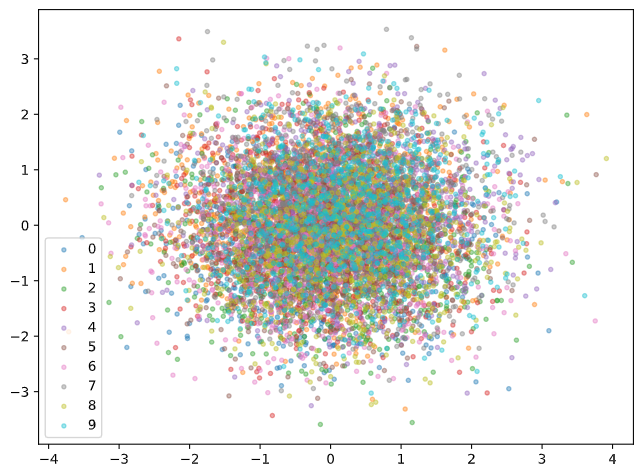
First two principal components of latent features from VAE.

It seems like VAE is actually not so useful for this task! Recall that one of the features of VAE is that our 64 dimensional latent feature space is composed of 64 independent Gaussian random variables. In addition, there is a regularization term penalizing terms that are too far away from the standard normal distribution. The result is we get a lot of independent principal components in the latent space, and thus using PCA to visualize the variance is not very useful. If we’re interested in reducing the variance in the data to just two latent dimensions, we may need to choose a lower dimensional embedding to train the VAE.

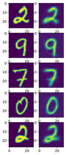
The reconstruction vs input image comparison is similar to the AE example. Qualitatively, the image background are less noiser, which could indicate that a more robust representation is learned. One interesting thing to note is that once the network is trained, unless we set a random seed, the reconstructed image will be different everytime, since the reconstruction depends on sampling from a Gaussian latent variable. We could sample many reconstructions from a single input to approximate the distribution of the reconstruction.

Original(left), VAE reconstruction(right) on MNIST

Conclusion

Hopefully someone finds this helpful to learn a little bit about VAE(and AE). VAE/AE is a really interesting topic and often these models are used as part of a larger machine learning system, learning representations that can be used to better train on other tasks. The first time I really ran into VAE was actually learning about latent ODE [4], which use VAE to encode the input into a low dimensional latent space, then learn continuous time dynamics on the latent space, and then use the decoder to map the continuous latent space to get a continuous time interpolation between points in the time series. The point is, VAE/AE is a very flexible deep learning tool.

References

[1] Oleksii Kuchaiev and Boris Ginsburg. Training Deep AutoEncoders for Collaborative Filtering.

[2] Diederik Kingma and Max Welling. Auto-Encoding Variational Bayes

[3] Carl Doersch. Tutorial on Variational Autoencoders.

[4] Ricky Chen, Yulia Rubanova, Jesse Bettencourt, David Duvenaud. Neural Ordinary Differential Equations