Some Simple PDEs Visualized Using Julia
This blog post is going to go over how to build Partial Differential Equation(PDE) solver from a novice perspective. One of the resources that inspired and helped me to write this is Solving PDEs in Julia by Chris Rackauckas, the lead dev on DifferentialEquations.jl. I highly recommend you check out his JuliaCon 2018 talk, which goes a lot more into depth on how to build a PDE solver out of components in DifferentialEquations.jl and other Julia libraries.
This was my first time both for working with differential equations in Julia and for writing a PDE solver. I chose to write a solver for the 1D heat and wave equations with Dirichlet boundary conditions, since they are the most straightforward and show up in every introductory PDE course. If you want to play around with the code it’s availble at tqhdesilva/pde-viz.
Quick Background on PDEs
Although it would be good to know some PDE before reading this, I don’t think it’s necessary to know the math to appreciate the visuals below. So here’s a quick background on PDE and the physical interpretation on the heat equation and wave equation.
Partial Differential Equations(PDE) are equations relating partial derivatives of a function. For example, if we have a function $u(x, t)$, representing the heat along a rod of length $L$ at time $t$ and position $x$, the distance from a given end, we could choose to represent our function with the equation:
\[u_t = u_{xx}\]where $u_t = \frac{\partial u}{\partial t}$ and $u_{xx} = \frac{\partial^2 u}{\partial x^2}$. To unambiguously define $u$, we also need initial conditions and boundary conditions. Initial condition is the heat distribution in the rod at time $0$:
\[u(x, 0) = f(x) \qquad \forall x \in (0, L)\]Boundary conditions are the temperature at the ends, where $x = 0$ or $x = L$. Today we are only going to use Dirichlet boundary conditions, which means the boundary conditions don’t vary over time.
\[\begin{align} u(0, t) & = K_1 \\ u(L, t) & = K_2 \end{align}\]The combination of the partial differential equation, initial condition, and boundary conditions is enough to determine the system.
Why Use Julia for Differential Equations?
Julia is a great programming language for scientific computing in general.
For differential equations in particular, there are some great libraries, notably
DifferentialEquations.jl which we used to write this post.
One downside to using Julia for differential equations is that some
libraries still need some polishing,
which is just a consequence of the Julia ecosystem not being mature yet.
For instance, while
working on this post
I found out that DifferentialEquations.jl doesn’t yet support stiff
solvers for second order ODE problems.
I also think that it’s a bit harder to debug Julia errors,
but maybe that’s because Julia is still new to me.
There’s also some libraries that are used to support research into the combination of neural networks and differential equations, such as NeuralNetDiffEq.jl and DiffEqFlux.jl. These libraries are a part of SciML, an open source project aimed at advancing scientific machine learning.
Heat Equation
The heat equation in 1D is commonly used to model an insulated rod with the ends connected to a heat source or sink held at a constant temperature. In general though, the heat equation can be used to model other types of diffusion. It can also be used to model how the probability density of a stochastic process(specifically a random walk) changes over time. You could even apply the higher dimensional case to denoising images.
The approach I used to solve the heat equation is the explicit method of the Finite Difference Method(FDM). The idea is to solve the equation
\[u_t = u_{xx}\]by solving for $u_t$ with the forward difference over $t$ and $u_{xx}$ with the second order central difference over $x$. The equality can be rewritten as:
\[\frac{u_j^{n + 1} - u_j^n}{\Delta t} = \frac{u_{j + 1}^n - 2 u_j^n + u_{j - 1}^n}{\Delta x^2}\]where $u_j^n$ is the value of $u$ at $t = \Delta t n$ and $x = \Delta x j$. We can write a recursion relation in time as:
\[u_j^{n + 1} = u_j^n + \frac{\Delta t}{\Delta x^2} (u_{j + 1}^n - 2 u_j^n + u_{j - 1}^n)\]We can reformulate this recursive relation using matrix multiplication:
\[\boldsymbol{u}^{n + 1} = \boldsymbol{u}^n + \frac{\Delta t}{\Delta x ^2 } \boldsymbol{A} \boldsymbol{u}^n + \boldsymbol{k}\]where $\boldsymbol{A}$ is a $ J \times J$ tridiagonal matrix when $J$ is the number of time steps $j$:
\[\boldsymbol{A} = \begin{bmatrix} -2 & 1 & & 0 \\ 1 & \ddots & \ddots & \\ & \ddots & \ddots & 1 \\ 0 & & 1 & -2 \\ \end{bmatrix}\]and the vector $\boldsymbol{k}$ accounts for the boundary conditions:
\[\boldsymbol{k} = \begin{bmatrix} K_1 \\ 0 \\ \vdots \\ K_2 \end{bmatrix}\]Case 1
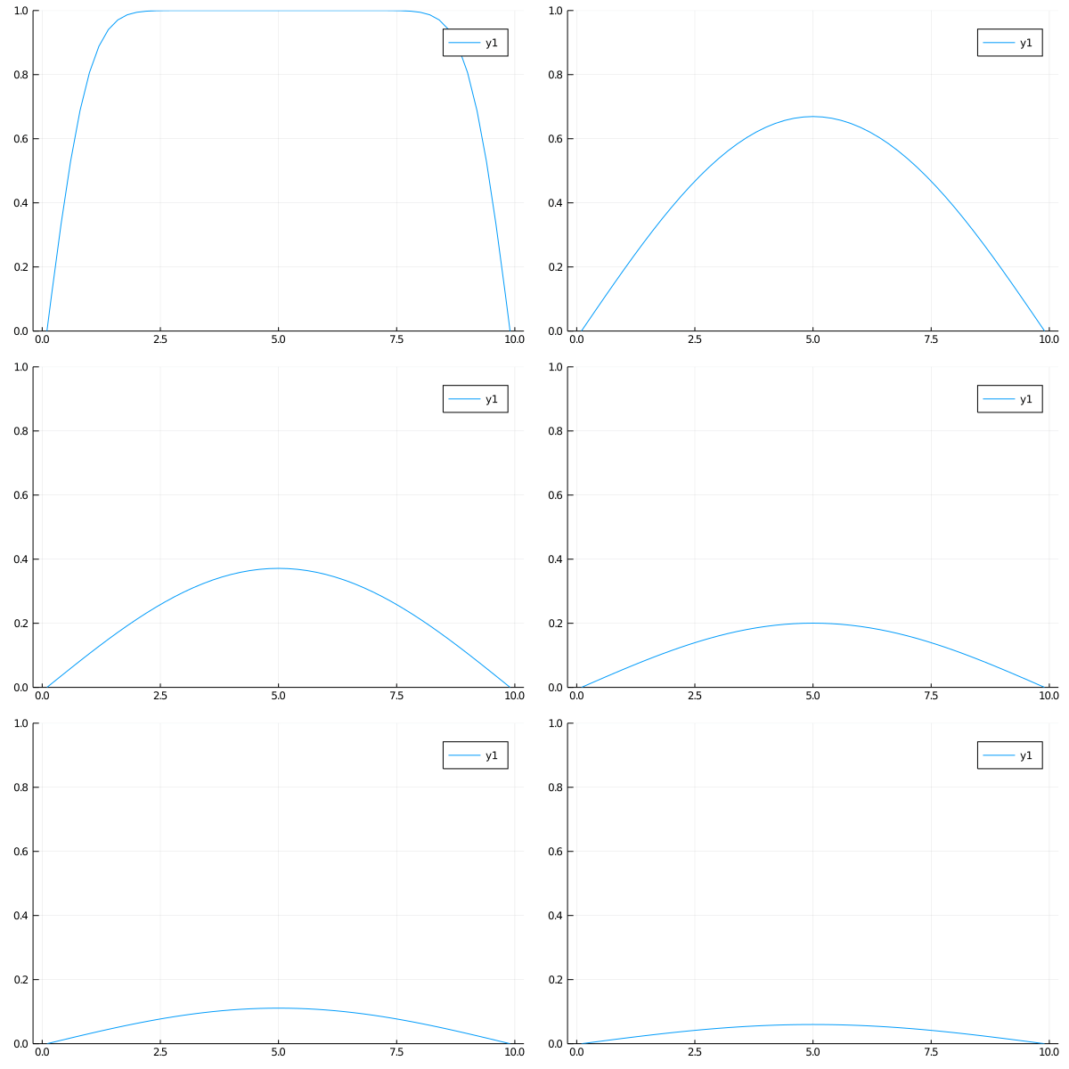
The first case for the heat equation is analogous to a cold insulated rod with the ends connected to a constant heat source. At first only the ends will heat up, but soon the heat will diffuse evenly and approach a uniformly heated rod.
\(\begin{align}
\qquad & u_t = u_{xx} \qquad & \forall x \in (0, 10),\: t \gt 0 \\
\qquad & u(0, t) = u(10, t) = 0 \qquad & t \gt 0 \\
\qquad & u(x, 0) = 0 \qquad & x \in (0, 10)
\end{align}\)
Case 2
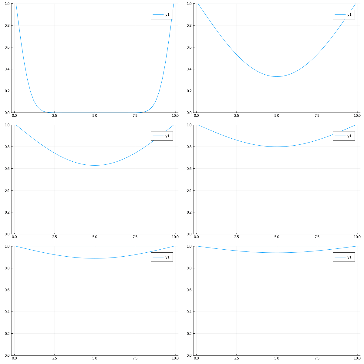
The second case is the opposite of the first case. This time an insulated rod at a uniform temperature is connected on the ends to two heat sinks. At first only the edges will cool significantly, but eventually the temperature in the rod will approach 0 everywhere.
\(\begin{align}
\qquad & u_t = u_{xx} \qquad & \forall x \in (0, 10),\: t \gt 0 \\
\qquad & u(0, t) = u(10, t) = 1 \qquad & t \gt 0 \\
\qquad & u(x, 0) = 1 \qquad & x \in (0, 10)
\end{align}\)
Case 3
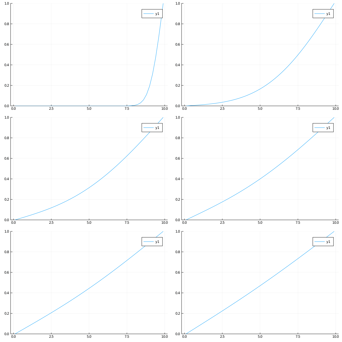
In this case we again have an insulated rod. The left end is a heat sink and the right end is a heat source, both held at the same temperature. The steady state of the rod occurs when the heat increases linearly moving from one end to the other.
\(\begin{align}
\qquad & u_t = u_{xx} \qquad & \forall x \in (0, 10),\: t \gt 0 \\
\qquad & u(0, t) = 0,\: u(10, t) = 1 \qquad & t \gt 0 \\
\qquad & u(x, 0) = 1 \qquad & x \in (0, 10)
\end{align}\)
Wave Equation
The wave equation can be used to describe phenomena such as a vibrating string, ocean waves, and quantum mechanics.
The general form of the wave equation is:
\[u_{tt} = c^2 u_{xx}\]where $c^2$ usually determines something analagous to how quickly the wave propagates in space.
I chose to solve the wave equation differently than the heat equation. Instead of calculating the forward difference in $t$, I chose instead to only apply FDM to the right side. Applying the forward difference here wouldn’t work on the left side, since the left term is now a second order partial derivative of $u$.
Calculating the right side is the same as before, using the second order central difference, but now we leave the left side as is:
\[\frac{\partial^2 u_j}{\partial t^2} = \frac{u_{j + 1} - 2 u_j + u_{j - 1}}{\Delta x^2} \\ \boldsymbol{u}_{tt} = \frac{1}{\Delta x^2} \boldsymbol{A} \boldsymbol{u} + \boldsymbol{k}\]where $\boldsymbol{A}$ and $\boldsymbol{k}$ are defined similarly as before. Now we just have to
solve second order ODE in $t$, which we are able to do with DifferentialEquations.jl
Case 1
This first case is a standing sine wave. The ends are fixed, and the initial condition is a sine function.
\[\begin{align} \qquad & u_{tt} = u_{xx} \qquad & \forall x \in (0, 10),\: t \gt 0 \\ \qquad & u(0, t) = u(10, t) = 0 \qquad & \forall t \gt 0 \\ \qquad & u(x, 0) = \sin (\frac{\pi x}{5}) \qquad & \forall x \in (0, 10) \\ \qquad & u_x(x, 0) = 0 \qquad & \forall x \in (0, 10) \end{align}\]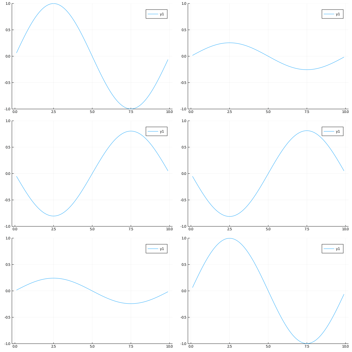
Case 2
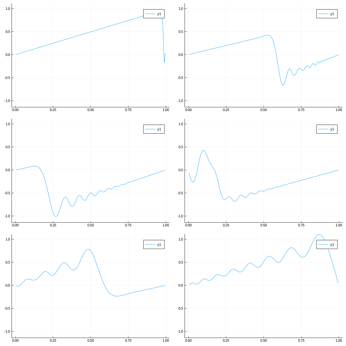
This one I pulled from a homework assignment. I’m not really sure what physical system this would correspond to.
\[\begin{align} \qquad & u_{tt} = 4 u_{xx} \qquad & \forall x \in (0, 10),\: t \gt 0 \\ \qquad & u(0, t) = u(10, t) = 0 \qquad & \forall t \gt 0 \\ \qquad & u(x, 0) = x \qquad & \forall x \in (0, 10) \\ \qquad & u_x(x, 0) = -x \qquad & \forall x \in (0, 10) \end{align}\]